Lab 2 Visual Odometry

Heads up!

Your official lab manual and Canvas rubric are the source of truth for deliverables and grading. Use this page to prepare faster, work smoother, and avoid the classic mistakes.

Quick reminder before you write that lab report:

• This site is public. If you found it, so can plagiarism checkers.
• Screenshotting a LaTeX derivation or re-typing it word for word is still copying.
• The whole point of these notes is that you understand the steps. If you can re-derive it without looking, you’re safe. If you can’t, you’re not ready to write it yet.
• “An Aggie does not lie, cheat or steal.” Your report should sound like you.

Overview

Lab 1 left you with a problem: everything you measured was in pixels. Pixels are not a real-world unitt, the same object measures a different number of pixels depending on how far it is from the camera. This lab fixes that.

Your team has two assignments. First, calibrate the tracking camera by finding a conversion factor between pixels and S.I. units (meters), with its own uncertainty. Second, use the calibrated camera to measure gravitational acceleration $g$ by tracking an object sliding down the tilted air table.

---

Before Lab

Concepts you need

Calibration by known reference: to convert pixels to meters, measure something whose real length you already know (e.g., with a meter stick). The conversion factor is:

$$k=\frac{L_{\text{real}}}{L_{\text{pixels}}}\left[\frac{\text{m}}{\text{px}}\right]$$

Both the real measurement and the pixel measurement carry uncertainty, so $k$ does too.

Propagation of error for division: the same quadrature rule from Lab 1 applies. For any $z=x/y$:

$$\frac{\delta z}{z}=\sqrt{{\left(\frac{\delta x}{x}\right)}^2+{\left(\frac{\delta y}{y}\right)}^2}$$

You’ll use this twice: once for the conversion factor $k$, and again at the end for $g$.

Kinematics chain: position, velocity, and acceleration are linked by derivatives:

$$\vec{v}(t)=\frac{d\vec{r}}{dt}\vec{a}(t)=\frac{d\vec{v}}{dt}$$

Your data comes as discrete frames, so in practice each derivative is a “change between frames divided by time between frames.” Expect the noise to grow with each derivative, acceleration data always looks messier than position data. This is normal.

Moving average: a moving average smooths noisy data by replacing each point with the average of itself and its two nearest neighbors. Random noise pushes points up and down at random, so averaging a small window cancels much of it out while keeping the real trend. For a 3-point centered window:

$$v_i^{\text{smooth}}=\frac{v_{i-1}+v_i+v_{i+1}}{3}$$

A larger window gives smoother data but blurs out real changes, so a small window like this is a good starting point.

Theory in practice

You don’t need the formula in a spreadsheet, AVERAGE over a sliding range does it for you. In a new column next to your data, average a window of the raw column, then drag the formula down. For example, if your velocity data is in column B starting at row 2:

=AVERAGE(B2:B4)

Place this in row 3 (the center of the window) and drag down. Each cell now averages the point above, the point itself, and the point below.

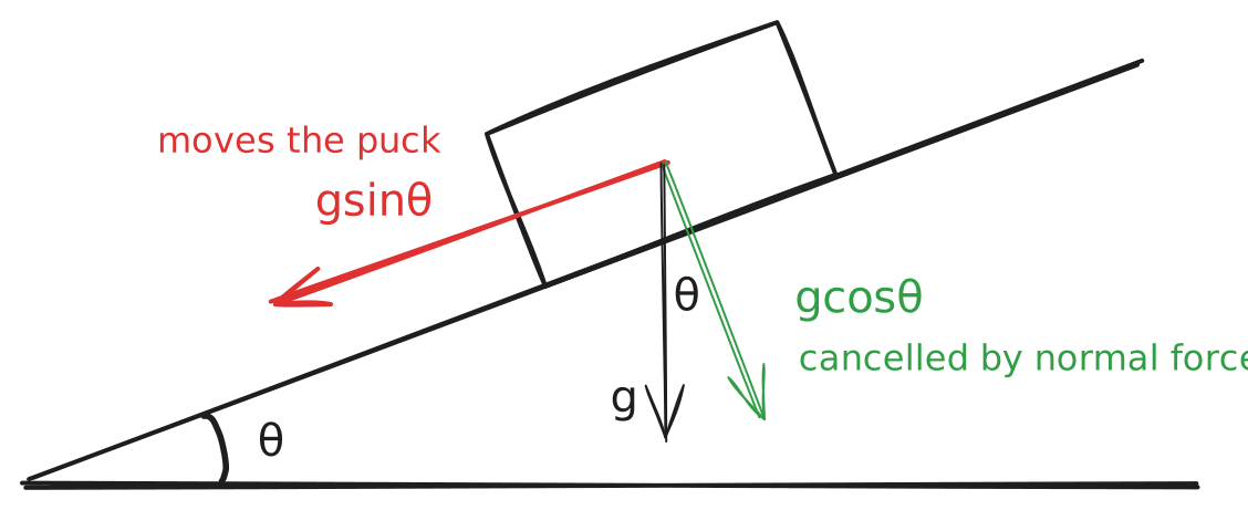
Incline physics: an object sliding down a frictionless incline at angle $\theta$ accelerates at $a=g\sin \theta$ along the slope. Rearranged:

$$g=\frac{a}{\sin \theta }$$

Why does an incline give us $g$?

Gravity pulls the puck straight down, but the puck can only move along the table’s surface. Only the part of gravity pointing along the incline actually accelerates it, and trigonometry says that part is $g\sin \theta$. So the puck slides with $a=g\sin \theta$, and measuring $a$ and $\theta$ lets you solve backwards for $g$.

Bonus: dropping something in free fall is too fast for the camera to track well. The incline slows the motion down to a measurable pace without changing the physics. The air table’s job is to make “frictionless” approximately true.

Theory in practice

If you find acceleration by fitting a straight line to your velocity data, Excel and Google Sheets both have a built-in function for the slope of a best-fit line.

• Excel SLOPE function
• Google Sheets SLOPE

Know before you walk in

• The air table tilts up to about 3.6°. The built-in inclinometer is most accurate at its extreme positions (0° or full tilt). Always set your incline to the full tilt for this experiment.
• $\sin \theta$ expects your angle in the right mode. Check whether your calculator or spreadsheet wants degrees or radians before lab, not during.
• Unlike Lab 1, the columns rx, ry, vx, vy, ax, and ay in your CSV now matter. They hold the position, velocity, and acceleration components of your tracked sticker.

---

During Lab

Linux Commands Cheatsheat

Common commands such as connecting to Jetson and working with files are outline in Getting Started with ENGR 216.

Commands you’ll use

Same workflow as Lab 1 — copy the script out of the write-protected directory, then run it:

cp examples/tracking/4_track_and_print_with_camera_input.py ~

python3 4_track_and_print_with_camera_input.py

Stop the recording with ⌃ Ctrl + C when your run is complete. If anything misbehaves, check Troubleshooting or ask a PT.

Procedure tips

• Calibrate first, in the same camera setup you’ll experiment with. Your conversion factor is only valid for that camera position and height. If the camera moves after calibration, recalibrate.
• Calibrate with a large known distance. Place two stickers a full meter-stick length apart rather than a few centimeters apart. The relative uncertainty of your conversion factor shrinks as the reference distance grows.
• Record calibration as a data set, not a single frame. Let the camera track the two stickers for a while, then average the pixel distance. This gives you the uncertainty on $L_{\text{pixels}}$ the same way you did in Lab 1.
• Release from rest, from the top, multiple times. Several clean slides give you multiple independent measurements of $a$, and a real uncertainty to report.
• Watch the camera feed for flickering. Same as Lab 1, if a color drops in and out, the lighting is insufficient. Look for a PT.

Troubleshooting

Symptom	Likely cause	Fix
Cannot connect with Jetson	Cable unplugged / loose	Unplug then plug in again. If problem prevails, ask a PT to change the cable.
Cannot connect with Jetson (MacOS)	Port not recognized	Change the to a different USB port and open a new terminal to connect.
Camera not detected	Cable unplugged / loose	Look for the USB connection between the camera and the table. Disconnect then connect again.
A sticker isn’t tracked or flickering tracking	Duplicate color, glare, not enough ligting, or sticker out of frame	Swap to an unused color; reposition to reduce glare; check the camera’s view; use an additional flashlight
Velocity or acceleration data looks very noisy	Derivatives amplify measurement noise	This is expected. Record longer slides and more trials, and report an average with uncertainty
Laggy video feed	Resource exhaustion	Restarting the camera by unplugging, or restarting Jetson. This is a slow process, ask a PT to move to an empty table.
Permission denied when script writes output	You’re running from the examples directory (write-protected)	Copy the script to your own folder first, run it there

Before you leave the lab

• Calibration data recorded: two stickers a known, measured distance apart, tracked over many frames
• Table angle recorded
• Multiple clean slides captured, each starting from rest
• CSV position, velocity, and acceleration columns are populated for your tracked sticker
• Every teammate has a copy of the lab data
• Have a PT sanity-check one of your velocity plots
• You can explain, in one sentence, how your conversion factor turns any pixel distance into meters. You’ll need to write exactly that in the report.

---

After Lab

What the deliverables are really testing

The two assignments split the grade roughly in half, and each half has a distinct point:

1. Calibration (description + equation) tests whether you understand that a measuring instrument is only as good as its calibration, and that the conversion factor is itself a measured quantity with an uncertainty you must evaluate and report. Your final equation should convert any pixel distance to meters, with the uncertainty of the factor stated explicitly.
2. Measuring $g$ (description, plots, acceleration, result) tests the full experimental chain: raw tracking data → calibrated positions → velocity → acceleration → a physical constant. The six plots ($x$ and $y$ components of $\vec{r}$, $\vec{v}$, $\vec{a}$ versus time) let the reader see that chain working.

A good sanity check: the accepted value of $g$ is about $9.81{\text{m/s}}^2$. If yours lands far away, revisit your angle, your units, and whether friction crept in; and if it still disagrees, discuss why in your report rather than hiding it. A well-explained discrepancy earns your team points, a suspiciously perfect number earns nothing.

Analysis checklist

• Compute the conversion factor $k$ and its uncertainty from your calibration data
• Convert your tracking data to S.I. units before (or while) computing anything physical
• Plot all six graphs: $x$ and $y$ components of position, velocity, and acceleration versus time, each with labeled axes and units
• Determine the average acceleration along the slide and its uncertainty
• Calculate $g=a/\sin \theta$, then propagate uncertainty from both $a$ and your angle measurement
• Report $g$ with its uncertainty and appropriate significant figures

Common mistakes that cost points

• No uncertainty on the conversion factor: the manual asks for it explicitly, in both the description and the equation
• Degrees/radians mix-up: $\sin (3.6)$ in radian mode is not $\sin (3.6°)$, and it will wreck your $g$ silently
• Mixed units: converting some quantities to meters but leaving others in pixels midway through the chain
• Missing plots or unlabeled axes: six plots are required, and every axis needs a label and a unit
• Ignoring the report template: still the easiest 10% you’ll ever earn or lose

---

Up next

You can now measure real-world motion in real-world units: position, velocity, and acceleration from nothing but a camera. You will use those knowledge to quantify the friction between a wooden and a metal surface, with varying contact areas and inclines.

Your next stop

Lab 3 Friction Force Evaluation